Traffic Simulator
Preparation
As I’m writing this blog about something I did almost 3 years ago, I’m having some trouble remembering the exact circumstances that led me to simulate traffic in a city. However, the general direction was that I was interested in measuring how certain parameters (speed-limit, driver reaction-time, vehicle density etc…) affect congestion (and btw, the definition of congestion is also not trivial).
So, the basic idea is to have some representation of a map - a graph of streets with various metadata, and on this map, vehicles would spawn, and follow some simple rules that model a driver (accelerate to meet the speed limit, decelerate/break when entering a junction or in response to a vehicle in front).
To start, I needed a playing field - a map. So I went to OpenStreetMap a pulled a map file of the Tel-Aviv area.
Parsing the map
The file is an XML file, and is pretty huge relative to the size of the area it represents. Mainly as it contains a lot of information that’s not relevant to the simulation (street names, buildings etc…).
What I really need (initially) are coordinates of streets. This can be obtained by parsing the <node> tags:
<node id="139698" lat="32.0938800" lon="34.7912317" version="19" timestamp="2011-12-12T17:34:51Z" changeset="10101015" uid="385027" user="Ori952"/>
What we care about are the node’s id, lon (longitude) and lat (latitude). Which can be parsed and stored into nodes like this:
with open('map.osm', 'rU') as xml_file:
    tree = etree.parse(xml_file)
    root = tree.getroot()
    nodes = {}
    ways = []
    for child in root:
        if child.tag == 'node':
            lon = float(child.get('lon'))
            lat = float(child.get('lat'))
            nodes[child.get('id')] = (lon, lat, )
The next type of information we need are the actual streets that connect the nodes. Those are represented by <way> tags:
<way id="5013379" version="16" timestamp="2014-11-15T12:53:09Z" changeset="26797570" uid="331840" user="yrtimiD">
    <nd ref="1628415541"/>                                                                                                                                                                       <nd ref="2470788072"/>
    <nd ref="2109540860"/>
    <tag k="highway" v="pedestrian"/>
    <tag k="int_name" v="Nahalat Binyamin"/>
    <tag k="motor_vehicle" v="no"/>
    <tag k="name" v="נחלת בנימין"/>
    <tag k="name:en" v="Nachalat Biniamin"/>
    <tag k="name:he" v="נחלת בנימין"/>
</way>
Initially, what we need is just the list of node ids that compose the road. However, there are two important points:
-
Not all
<way>s represent vehicle roads. This is determined by thev(value) property of the<tag>whosek(key) ishighway:NON_ROAD_TYPES = ['proposed', 'platform', 'path', 'footway', 'pedestrian', 'cycleway', 'road', 'steps', 'track', 'unclassified', 'construction'] def way_of_road(way): for child in way: if child.tag == 'tag' and child.get('k') =='highway': if child.get('v') in NON_ROAD_TYPES: return False return True return False -
Some roads are two-way. As our graph will be directed, we need to manually add the arcs in the opposite direction.
Eventually we can parse the road data into the ways list using:
for child in root:
    if child.tag == 'way':
        way = child
    if not way_of_road(way):
        continue
    nds = []
    for nd in way:
        if nd.tag == 'nd':
            nds.append(nd.get('ref'))
    ways.append((nds, speed))
    if two_way_road(way):
        ways.append((list(reversed(nds)), speed))
Now, we’re almost there, as we have a list of “ways” which are themselves lists of nodes. But what we actually need is arcs, which are tuples of consecutive nodes:
ref_arcs = []
for way in ways:
    arc_tuples = zip(way[:-1], way[1:])
    ref_arcs.extend((src, dst) for src, dst in arc_tuples)
Refining
If you think about it, the map file we use is a cropped map. So what would happen is that we will have lots of roads that leave or exit the map that are dead-end. If we don’t want our map to have car sinks, we need to eliminate all those dead-ends:
while True:
    src_set = set(src for src, _, _ in ref_arcs)
    _ref_arcs = []
    discarded = False
    for src, dst, speed in ref_arcs:
        if dst in src_set:
            _ref_arcs.append((src, dst, speed))
        else:
            discarded = True
    # If no arcs were discarded in this round we are done
    if not discarded:
        break
    ref_arcs = _ref_arcs
Coordinates
The node coordinates are all angular - longitude and latitude. However, on the ground, vehicles are moving at km/h (or m/s). We have no way of running the simulation without assigning fixed coordinated to the nodes.
There is an entire science to measuring the earth. But I wanted to choose something simple.
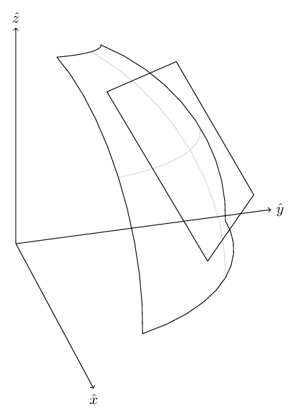
Basically what I did was take the lon/lat bounding box the of map. This describes a part of the earth’s shell:
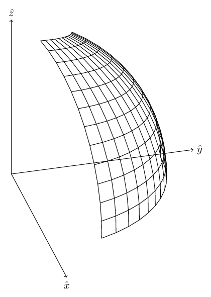
Now, we draw a plane tangent to the earth at the center of that “shell”:
Now, suppose we have a point $ \vec E$ on the earth’s surface:
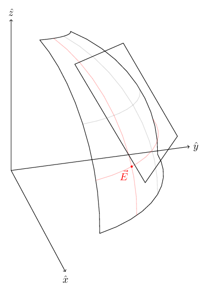
We will cast a ray from the center of the earth to that point, and continue tracing it until it intersects with the plane (or map if you will) at $ \vec M$ :
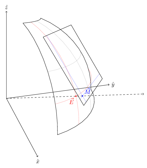
We now have a 1-to-1 mapping from points on the surface of the earth to points on a flat map!
Now we need a way to get 2D coordinates. To do that we need to select axes.
We start with a north “hint”, we can use the $\hat z $ vector as it points at the north pole. Obviously, this vector does not fit in map, but sticks out of it. We want to take the component of $\hat z $ that’s embedded in the map and use that as “north”. Generally, a vector can be decomposed in relation to a plane to a perpendicular (in the direction of the plane’s normal) and transverse (embedded in the plane, and thus perpendicular to the normal) $\hat z $ :
\[\hat z = \vec z_{\parallel} + \vec z_{\bot}\]Since $\vec z_{\parallel} $ is perpendicular to $\hat n $ , then $\vec z_{\parallel} \cdot \hat n = 0 $ .
In addition, $\vec z_{\bot} $ is in the direction of $\hat n $ , so we can write it as: $\vec z_{\bot} = \alpha \hat n $
We can now use all that to extract $\vec z_{\parallel} $ (which will serve as the plane’s north):
\[\begin{eqnarray*} \hat z \cdot \hat n & = & \vec z_{\parallel} \cdot \hat n + \vec z_{\bot} \cdot \hat n & = & \alpha \end{eqnarray*}\]On the surface of the map, we can have east/north axis and thus a 2D coordinate system.
So, first, I want to convert lon/lat coordinates to a 3d point on the surface of earth’s sphere. These are just Spherical Coordinates:
\[\hat{r}(lon, lat) = (\cos(\theta) \cos(\phi), \cos(\theta) \sin(\phi), \sin(\theta))\]def vector3_from_lon_lat(lon, lat):
l = lon * math.pi / 180
p = lat * math.pi / 180
return (math.cos(p) * math.cos(l), math.cos(p) * math.sin(l), math.sin(p))
What this would give us is the normal to the tangent plane: $\hat n_0 = \hat r(\frac{\pi}{180}lon, \frac{\pi}{180}lat)$. Which will give us the following equation for the tangent plane:
\[\vec r \cdot \hat n_0 = \hat r_0 \cdot \hat n_0 = R_E\]# Bounding box
minlon = min(lon for lon, lat in nodes.values())
maxlon = max(lon for lon, lat in nodes.values())
minlat = min(lat for lon, lat in nodes.values())
maxlat = max(lat for lon, lat in nodes.values())
# Center point
lon_0 = (minlon + maxlon) / 2
lat_0 = (minlat + maxlat) / 2
n_0 = vector3_from_lon_lat(lon_0, lat_0)
Now we can take the $\hat z$ and project it onto the tangent plane to get a “north” vector:
\[\vec N = \hat z - \left(\hat z \cdot \hat n_0\right) \hat n_0\]z = (0, 0, 1) # "real" north: points to the north pole
north_0 = sub3(z, scale3(n_0, dot3(z, n_0))) # Project north onto the tangent plane
north_0 = scale3(north_0, 1 / norm3(north_0)) # Normalize
East is then obtained by using a cross product (right-hand rule):
\[\hat E = \hat N \times \hat n_0 = \frac{\vec N}{\left\Vert\vec N\right\Vert} \times \hat n_0\]east_0 = cross3(north_0, n_0) # Right-hand rule
The north and east facing unit-vectors on the plane will be used as basis vectors.
Now for each lon/lat coordinate, we scale it using earth’s radius (6.317e6[m]) towards the plane:
\[\vec r (t) = t \hat r (\theta, \phi)\]If we plug this into the equation for the tangent plane:
\[\left(t \hat r (\theta, \phi)\right) \cdot \hat n_0 = R_E \Rightarrow t = \frac{R_E}{\hat r (\theta, \phi) \cdot \hat n_0}\]Which gives us the following intersection point on the plane:
\[\vec r = \frac{R_E}{\hat r (\theta, \phi) \cdot \hat n_0} \hat r (\theta, \phi)\]We can then decompose to north and south coordinates (in meters!):
n = vector3_from_lon_lat(lon, lat)
t = R_E / dot3(n, n_0)
x = scale3(n, t)
u = dot3(x, north_0)
v = dot3(x, east_0)
That’s it so far, next time we’ll talk about setting up a simulation.