A survey of Linear Programming

In the recent article about the internship lottery, we’ve formulated trading optimization in the following manner:

\[\begin{eqnarray} \mathrm{maximize} \ & \Delta = \sum_{i \in \mathcal{H}} \left(w_{\pi_A(i)} - w_{\pi_B(i)}\right) \left(x^+_i - x^-_i\right) \\ \mathrm{such\ that} & \sum_{i \in \mathcal{H}} w_{\pi_A(i)} \left(x^+_i - x^-_i\right) \ge 0 \\ & \sum_{i \in \mathcal{H}} w_{\pi_B(i)} \left(x^-_i - x^+_i\right) \ge 0 \\ & \sum_{i \in \mathcal{H}} \left( x^+_i - x^-_i \right) = 0 \\ & 0 \le x^-_i \leq \min\left\lbrace p_{A,i}, 1 - p_{B,i} \right\rbrace \\ & 0 \le x^+_i \leq \min\left\lbrace p_{B,i}, 1 - p_{A,i} \right\rbrace \end{eqnarray}\]

This is what’s called a linear programming problem, as were trying to optimize a linear function on some variables, given a set of linear constraints on said variables.

I’m going to try and do my best to explain what linear programming is, and how to approach solving them. There are many sources out there, and personally, I didn’t find one definitive source, but rather collected bits of insight which I’ll try to highlight here.

First, let’s try to give a generic formulation of the lottery optimization problem.

Formulation of linear optimization

We will break up the linear optimization in two parts:

1. The problem domain, meaning the possible values that the variables can take based on the constraints. Also knows as the feasible region.
2. The cost function, and the type of optimum (minimum/maximum).

We will examine each separately, and then combine the various properties of each to reach an algorithm that can give us a solution.

First of all, let’s take all the variables (suppose there are n of them) and serialize them into one vector $\mathbf{x} \in \mathbb{R}^n$.

Now, the constraints can be written in terms of $\mathbf{x}$, and we can notice three types of constraints:

\[\begin{eqnarray} \mathbf{a}^T \mathbf{x} \le b \\ \mathbf{a}^T \mathbf{x} \ge b \\ \mathbf{a}^T \mathbf{x} = b \end{eqnarray}\]

The two inequality constraints are actually equivalent, as we can transform them by negation:

\[\mathbf{a}^T \mathbf{x} \ge b \Rightarrow -\mathbf{a}^T \mathbf{x} \le -b\]

The equality constraint can similarly be written as two complementary inequality constraints:

\[\mathbf{a}^T \mathbf{x} = b \Rightarrow \begin{cases} \mathbf{a}^T \mathbf{x} \le b \\ \mathbf{a}^T \mathbf{x} \ge b \end{cases}\]

So we could write all constraints in terms of inequality only, and sometimes this will serve us, but more commonly we will have two types of constraints: inequality (of just one kind) and equality. Let’s write them all down:

\[\begin{eqnarray} \mathbf{a}_1^T \mathbf{x} & \le & b_1 \\ \ldots \\ \mathbf{a}_l^T \mathbf{x} & \le & b_l \\ \mathbf{a}_{l+1}^T \mathbf{x} & = & b_{l+1} \\ \ldots \\ \mathbf{a}_m^T \mathbf{x} & = & b_m \end{eqnarray}\]

As you can see, we have a total of m constraints, l of which are inequality constraints, and the rest are equality constraints.

Polyhedrons

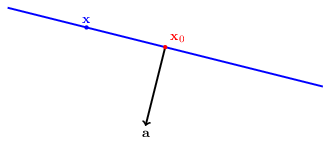
Each of the two types of constraints has a geometric interpretation in n-dimentional space. for some vector $\mathbf{x}_0 \in \mathbb{R}^n$ and a vector $\mathbf{a} \in \mathbb{R}^n$:

• A hyperplane (blue line) is the set of all vectors $\mathbf{x} \in \mathbb{R}^n$ which satisfy $\mathbf{a}^T \mathbf{x} = \mathbf{a}^T \mathbf{x}_0 \left(=b\right)$.

  

• A halfspace (grayed area) is defined by all vectors $\mathbf{x} \in \mathbb{R}^n$ which satisfy $\mathbf{a}^T \mathbf{x} \le \mathbf{a}^T \mathbf{x}_0 \left(=b\right)$:

  

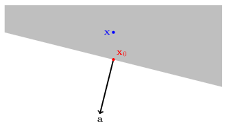
  In other words, all the vectors on the side on $\mathbf{x}_0$ that is in the opposite direction of $\mathbf{a}$.

Let’s make a notation for hyperplanes and halfspaces to match each constraint:

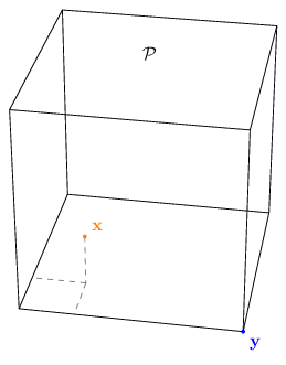
\[\begin{eqnarray} \mathcal{S}_i = \left\lbrace\mathbf{x} \in \mathbb{R}^n : \mathbf{a}_i^T \mathbf{x} \le b_i \right\rbrace \\ \mathcal{T}_i = \left\lbrace\mathbf{x} \in \mathbb{R}^n : \mathbf{a}_i^T \mathbf{x} = b_i \right\rbrace \end{eqnarray}\]

A polyhedron $\mathcal{P}$ is basically an intersection of a collection of hyperplanes and halfspaces:

\[\mathcal{P} = \mathcal{S}_1 \cap \ldots \cap \mathcal{S}_l \cap \mathcal{T}_{l+1} \cap \ldots \cap \mathcal{T}_m\]

Play around with the following demo to get a hang of polyhendrons. On the left is a plot of a 2D vector space, while on the right are a bunch of constraints you can toggle on/off by clicking. A red pixel on the plot means it’s in the polyhedron (in the intersection of the constraints).

What I want you to take from this demo is that:

1. Polyhedrons can be of any dimension - they can be areas (2D), line segments (1D) or even single points (0D).
2. It is possible that the polyhedron is empty, i.e. no point can be found to match all constraints.

In addition to those takes, it might be apparent from the demo that polyhedrons have endpoints. As it happens, polyhedrons can be described in terms of their endpoint in a way that’s useful to our end goal. Let’s turn our discussion to endpoints.

Vertices, Convex-Combinations and Extreme-points

So, let’s think how can we characterize the vertex (the formal name for endpoints) of polyhedrons. We can say a vector is a vertex if we can find a hyperplane which passes through that vertex, that does not intersect the polyhedron anywhere but the vertex.

The formal definition is that $\mathbf{x} \in \mathcal{P}$ is a vertex if we can find a $\mathbf{c} \in \mathbb{R}^n$ such that for any other vector $\mathbf{x} \neq \mathbf{y} \in \mathcal{P}$ we have $\mathbf{c}^T \mathbf{x} > \mathbf{c}^T \mathbf{y}$.

There’s another definition that’s equivalent, but requires the introduction of convex sums.

A convex sum or convex combination of vectors is a linear combination where the coefficients sum up to 1:

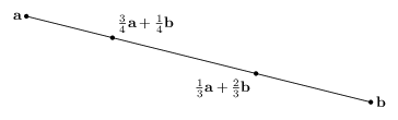
\[\lambda_1 \mathbf{x}_1 + \ldots + \lambda_k \mathbf{x}_k \quad : \quad \lambda_1 + \ldots + \lambda_k = 1\]

Intuitively, for two vectors $\mathbf{x}, \mathbf{y}$, their convex combination is just the line segment that connects them:

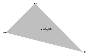
For three vectors, it would be the triangle area that’s formed by them:

Now, formally, a vector $\mathbf{x} \in \mathcal{P}$ is exteme if there are no two other vectors $\mathbf{y}, \mathbf{z} \in \mathcal{P}$ such that $\mathbf{x} \in \mathcal{P}$ is a convex combination of them.

So for the line segment, $\mathbf{a}$ can not be expressed as the (trivial) convex sum of $\mathbf{b}$, and in the triangle, $\mathbf{c}$ can not be expressed as the convex sum of $\mathbf{a}$ and $\mathbf{b}$ (because the convex sum of $\mathbf{a}$ and $\mathbf{b}$ can only be the line segment connecting them).

Unsurprisingly, the definition of a vertex coincides with that of an extreme point (there’s a proof, but I won’t go into it).

Now here’s the important bit. As it turns out, polyhedrons can be expressed as a collection of all the convex combinations of it’s vertices. Suppose that for a polyhedron $\mathcal{P}$ we managed to list all vertices V, then:

\[\mathcal{P} = \left\lbrace \sum_{v \in V} \lambda_v v : \sum_{v \in V} \lambda_v = 1 \right\rbrace\]

I will not show the entire proof here, just the intuition. The proof is by induction.

For the purpose of this discussion, we will define a polyhedron using a combination of halfspaces only (we already know this is possible):

\[\mathcal{P} = \left\lbrace \mathbf{x} \in \mathbb{R}^n : \mathbf{a}_i^T \mathbf{x} \le b_i, \quad i=1,\ldots,m \right\rbrace\]

We observe that a polyhedron is embedded in an affine-subspace (a face is embedded in a plane, a segment is embedded in a line), and we can define the dimension of a polyhedron as the dimension of the smallest affine-subspace that contains it.

Starting with a polyhedron that contains just one vertex. By definition, it’s a trivial convex combination of itself. So the claim holds. It’s also a polyhedron of dimension 0. This way we establish the base case.

Now, the induction step. We start with an assumption that a polyhedron of dimension up to k-1 is a convex combination of its vertices, and we are looking at a polyhedron of dimension k.

We then pick some vector $\mathbf{x}$ in the polyhedron that is not a vertex (otherwise it’s trivial), and a vector $\mathbf{y}$ that is a vertex.

Next, we cast a ray from $\mathbf{x}$ in the direction opposite to $\mathbf{y}$:

\[\mathbf{u} = \mathbf{x} + \lambda \left(\mathbf{x} - \mathbf{y}\right)\]

This ray must violate one the constraints as it leaves the polyhedron. Let’s say it violates constraint j ($\mathbf{a}_j = \left(0, -1, 0\right),\ b_j = 1$):

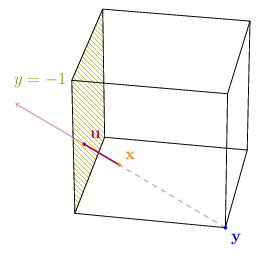
We then define an auxiliary polyhedron by turning the j^th constraint to an equality constraint.

\[\mathcal{Q} = \left\lbrace \mathbf{x} \in \mathcal{P} : \mathbf{a}_j^T \mathbf{x} = b_j \right\rbrace\]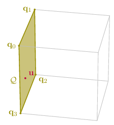

Without going into the proof, the resulting polyhedron will be of a lower dimension, therefore the induction premise holds and we can say that the intersection vector of the ray with the auxiliary polyhedron is a convex combination of its vertices:

\[\mathbf{u} = \sum \lambda_i \mathbf{q}_i\]

In addition, $\mathbf{x}$ can be written as some combination of the vertex $\mathbf{y}$ and the intersection $\mathbf{u}$:

\[\mathbf{x} = \frac{\mathbf{u} + \lambda \mathbf{y}}{1 + \lambda}\]

Now, it can be shown that every vertex of $\mathcal{Q}$ is a vertex of $\mathcal{P}$, and so, if we replace $\mathbf{u}$ with its convex sum, and rearrange a bit:

\[\begin{eqnarray} \mathbf{x} & = & \frac{\sum \lambda_i \mathbf{q}_i + \lambda \mathbf{y}}{1 + \lambda} \\ & = & \frac{\lambda}{1 + \lambda} \mathbf{y} + \sum \frac{\lambda_i}{1 + \lambda} \mathbf{q}_i \end{eqnarray}\]

We find that $\mathbf{x}$ is a convex combination of vertices of $\mathcal{P}$!

Maximizing over a polyhedron

It’s time we take a look at the second part of LP problems - the cost function.

Let’s examine the properties of the product $\mathbf{c}^T \mathbf{x}$ in the context of a polyhedron $\mathcal{P}$ with vertices $V_\mathcal{P} = \left\lbrace \mathbf{x}_1, \ldots, \mathbf{x}_N \right\rbrace$.

In the previous section I stated that each vector in a polyhedron is some convex combination of its vertices:

\[\begin{eqnarray} \mathbf{x} = \sum \lambda_k \mathbf{v}_k \\ \sum \lambda_k = 1 \end{eqnarray}\]

Let’s expand the product:

\[\mathbf{c}^T \mathbf{x} = \sum \lambda_k \mathbf{c}^T \mathbf{v}_k\]

Now, there are two options:

1. They all have the same product:

   \[\mathbf{c}^T \mathbf{v}_k = v\]

   In this case:

   \[\mathbf{c}^T \mathbf{x} = \sum \lambda_k \mathbf{c}^T \mathbf{v}_k = v \sum \lambda_k = v\]

   Which means the product with any vector in the polyhedron is the same as the vertices.

2. We can choose a vertex that gives the biggest product, and one that gives the smallest:

   \[\mathbf{c}^T \overline{\mathbf{v}} \ge \mathbf{c}^T \mathbf{v}_k \ \forall \ \mathbf{v}_k \in V_\mathcal{P} \\ \mathbf{c}^T \underline{\mathbf{v}} \le \mathbf{c}^T \mathbf{v}_k \ \forall \ \mathbf{v}_k \in V_\mathcal{P} \\\]

   In this case:

   \[\mathbf{c}^T \mathbf{x} = \sum \lambda_k \mathbf{c}^T \mathbf{v}_k \ge \sum \lambda_k \mathbf{c}^T \underline{\mathbf{v}} = \mathbf{c}^T \underline{\mathbf{v}} \sum \lambda_k = \mathbf{c}^T \underline{\mathbf{v}}\]

   And in a similar manner:

   \[\mathbf{c}^T \mathbf{x} \le \mathbf{c}^T \overline{\mathbf{v}}\]

   Or to sum it up:

   \[\mathbf{c}^T \underline{\mathbf{v}} \le \mathbf{c}^T \mathbf{x} \le \mathbf{c}^T \overline{\mathbf{v}}\]

   Which means one of the vertices has a more optimal product.

Both cases lead to the following concolusion: In a polyhedron, a linear function will have optimal values at the vertices.

So the problem of optimizing on a polyhedron boils down to finding all the vertices of a polyhedron, then selecting the one for which the cost is optimal:

\[\mathbf{x} = \underset{\mathbf{v} \in V_\mathcal{P}}{\mathrm{argmin}} \ \mathbf{c}^T \mathbf{v}\]

Basic feasible solution

Now is the time to discuss how to find the vertices of a polyhedron.

We first need to introduce a new definition: basic feasible solution (or BFS).

Consider a polyhedron $\mathcal{P}$ defined in terms of a mix of inequality and equality constraints $\left(\mathbf{a}_i, b_i\right)$:

\[\mathbf{a}_i^T \mathbf{x} \le b_i,\quad i \in I_\le \\ \mathbf{a}_i^T \mathbf{x} = b_i,\quad i \in I_=\]

A vector $\mathbf{x} \in \mathbb{R}^n$ is a basic solution if:

1. All equality constraints hold: $\forall i \in I_=,\quad \mathbf{a}_i^T\mathbf{x} = b_i$
2. Out of all constraints that satisfy $ \mathbf{a}_i^T \mathbf{x} = b_i $, there are n which are linearly-independant.

A basic solution $\mathbf{x} \in \mathbb{R}^n$ is a basic feasible solution if it satisfies all constraints.

Not surprisingly, a basic feasible solution is equivalent to a vertex.

Polyhedron in standard form

We will now explore polyhedron of a specific form:

\[\mathcal{P} = \left\lbrace \mathbf{x} \in \mathbb{R}^n : \mathbf{A}\mathbf{x} = \mathbf{b}, \quad \mathbf{x} \ge 0 \right\rbrace\]

Where $\mathbf{A} \in \mathbb{R}^{m \times n}$ and $\mathbf{b} \in \mathbb{R}^m$. This gives us m equality constraints, and n inequality constraints.

Now, for a vector to qualify as a basic solution, we have to satisfy all the equality constraints, that’s m. We need an additional n-m constraints to form a set of vectors that are linearly independant. But all we have left are inequality constraints. So we “cast” them to equality constraints (as the definition allows). If all the components of the resulting solution are positive, this would give us a basic feasible solution.

That was the handy-wavey explanation. The algorithm for finding a basic solution is as follows:

1. Select some subset of m linearly independant columns of $\mathbf{A}$:

   \[\mathbf{B} = \left(\mathbf{A}_{\beta(1)}, \ldots, \mathbf{A}_{\beta(m)}\right)\]

   There could be many such choices of $\beta: [1,m] \rightarrow [1,n]$.

2. For every $i \notin \mathrm{Im}\beta$ we set $x_i = 0$
3. Solve the equation system \(\mathbf{B}\mathbf{x}_\beta = \mathbf{b}\) to obtains $x_{\beta(1)},\ldots,x_{\beta(m)}$.

Brute-Force Approach

We already know enough to write down a brute force algorithm for solving LP.

Given an LP in standard form:

\[\mathcal{P} = \left\lbrace \mathbf{x} \in \mathbb{R}^n : \mathbf{A}\mathbf{x} = \mathbf{b}, \quad \mathbf{x} \ge 0 \right\rbrace \\ \tilde{\mathbf{x}} = \underset{\mathbf{x} \in \mathcal{P}}{\mathrm{argopt}} \ \mathbf{c}^T\mathbf{x}\]

We know the solution is actually:

\[\tilde{\mathbf{x}} = \underset{\mathbf{x} \in V_\mathcal{P}}{\mathrm{argopt}} \ \mathbf{c}^T\mathbf{x}\]

Or, in Python:

import itertools
import numpy as np

def costs(A, b, c) -> iter[tuple[np.array, float]]:
    m, n = A.shape
    for beta in itertools.combinations(range(n), m):
        B = A[beta]
        if np.linalg.det(B) == 0:
            continue
        x = np.zeros(n)
        x[beta] = B.I @ b
        if x >= 0:
            yield x, c.T @ x

def optimize(A, b, c, opt=max) -> tuple[np.array, float]:
    return opt(costs(A, b, c), key=itemgetter(1))

However, the possible number of basic feasible solutions of a polyhendron is ${n \choose m}$ which is exponential!!! So clearly, not a very effective approach.

Luckily, there are better approaches to solving LP, which we will explore in the next few articles.

Summary

So we started out with a real-world optimization problem we want to solve.

We then went ahead and formulated it, and saw that it can be visualized geometrically using polyhedrons.

After exploring the properties of polyhedrons, we found out that we are interested in the vertices, because that’s where we will find an optimum.

However, we were still not close to a solution, because there’s no reasonable way to calculate the vertices.

Then we introduced the standard form, and basic feasible solutions, and saw there’s an easy algorithm to find them. But the algorithm is brute-force and very inefficient.

Next time, we’ll dive into that most famous algorithm for solving LP effciently - the Simplex Algorithm.